Linear Elasticity Convergence Study: Unit Square with Circular Hole
This demo is implemented in demo_elasticity_convergence.py. It
illustrates:
How to perform a convergence study for the linear elasticity problem on an unfitted domain.
How to use Nitsche’s method for imposing boundary conditions weakly.
How to compute and analyze L² and H¹ error norms for vector fields.
How to visualize convergence rates for different mesh refinements.
Problem Definition
We consider the linear elasticity problem on a domain \(\Omega \subset \mathbb{R}^2\) that is the unit square \([0,1]^2\) with a circular hole. The domain is defined implicitly as the complement of a disk:
where \(D_R(\mathbf{c})\) is a disk of radius \(R = 0.2\) centered at \(\mathbf{c} = (0.5, 0.5)\). The linear elasticity problem reads:
where \(\mathbf{u}\) is the displacement field, \(\mathbf{f}\) is the body force, \(\mathbf{g}\) is the traction force, and \(\mathbf{n}\) is the outward unit normal. The stress tensor \(\sigma(\mathbf{u})\) is related to the strain tensor \(\varepsilon(\mathbf{u})\) by the constitutive relation:
where \(\mu\) and \(\lambda\) are the Lamé parameters, and the strain tensor is:
The outer boundary (four edges of the square) forms the Dirichlet boundary \(\Gamma_D\), and the unfitted boundary (circular hole) is \(\Gamma_N\).
Boundary Conditions
We have two options for imposing boundary conditions on the unfitted boundary \(\Gamma_N\):
Neumann boundary conditions: Impose \(\sigma(\mathbf{u}) \cdot \mathbf{n} = \mathbf{g}\) directly in the linear form.
Nitsche’s method: Weakly impose Dirichlet boundary conditions \(\mathbf{u} = \mathbf{u}_D\) on \(\Gamma_N\) using Nitsche’s method.
Nitsche’s Method for Elasticity
When using Nitsche’s method, the bilinear form is modified to include boundary terms:
where \(\beta > 0\) is a stabilization parameter (chosen here as \(\beta = 30 k^2\) for polynomials of degree \(k\)), and \(h\) is the mesh size. The boundary terms ensure consistency, symmetry, and stability.
Manufactured Solution
We use the manufactured solution:
which yields a non-zero body force \(\mathbf{f}\) and non-zero traction on the boundary. The corresponding stress field is computed from the constitutive relation, and the body force is derived as \(\mathbf{f} = -\nabla \cdot \sigma(\mathbf{u})\).
Convergence Analysis
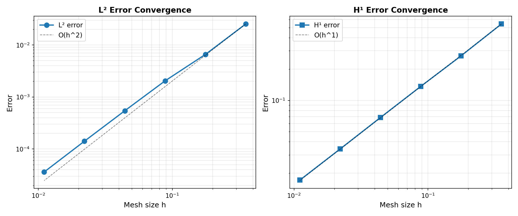
For a finite element solution \(\mathbf{u}_h\) using polynomial basis functions of degree \(k\), the expected convergence rates are:
L² error: \(\|\mathbf{u} - \mathbf{u}_h\|_{L^2(\Omega)} = \mathcal{O}(h^{k+1})\)
H¹ error: \(\|\mathbf{u} - \mathbf{u}_h\|_{H^1(\Omega)} = \mathcal{O}(h^k)\)
where \(h\) is the characteristic mesh size. These rates hold for smooth solutions when the mesh is sufficiently refined.
Implementation
Modules import
First we import the necessary modules:
from pathlib import Path

from mpi4py import MPI

import dolfinx.fem
import dolfinx.fem.petsc
import dolfinx.io
import numpy as np
import ufl

import qugar
import qugar.impl
from qugar.dolfinx import ds_bdry_unf, mapped_normal
from qugar.mesh import create_unfitted_impl_Cartesian_mesh
from qugar.utils import has_FEniCSx, has_PETSc

try:
    import matplotlib.pyplot as plt

    has_matplotlib = True
except ImportError:
    has_matplotlib = False

if not has_FEniCSx:
    raise ValueError("FEniCSx installation not found, required for this demo.")
if not has_PETSc:
    raise ValueError("petsc4py installation not found, required for this demo.")
Domain Definition
We define the domain as the unit square with a circular hole:
xmin = np.array([0.0, 0.0], dtype=np.float64)
xmax = np.array([1.0, 1.0], dtype=np.float64)
center = (xmin + xmax) / 2.0
R = 0.2

dtype = np.float64
impl_func = qugar.impl.create_negative(qugar.impl.create_disk(R, center=center))
Material Parameters
Define the material properties:
# Young's modulus and Poisson's ratio
E = 1.0
nu = 0.3

# Lamé parameters
mu = E / (2.0 * (1.0 + nu))
lmbda = E * nu / ((1.0 + nu) * (1.0 - 2.0 * nu))

print(f"Young's modulus E = {E}")
print(f"Poisson's ratio ν = {nu}")
print(f"Lamé parameter μ = {mu:.4f}")
print(f"Lamé parameter λ = {lmbda:.4f}")
Boundary Condition Method
Choose between Nitsche’s method (True) or Neumann boundary (False) conditions:
use_Nistche = True
Analytical Solution
Define the exact displacement solution:
def epsilon_expr(u):
    """Strain tensor."""
    return ufl.sym(ufl.grad(u))


def sigma_expr(u):
    """Stress tensor."""
    # Get spatial dimension from the mesh (2D in this case)
    # For a 2D problem, Identity(2) creates a 2x2 identity tensor
    return 2.0 * mu * epsilon_expr(u) + lmbda * ufl.tr(epsilon_expr(u)) * ufl.Identity(2)


def u_exact_expr(x):
    """Exact displacement solution as a UFL expression."""
    u1 = ufl.sin(ufl.pi * x[0]) * ufl.sin(ufl.pi * x[1])
    u2 = ufl.sin(ufl.pi * x[0]) * ufl.sin(ufl.pi * x[1])
    return ufl.as_vector([u1, u2])


def u_exact_numpy(x):
    """Exact displacement solution as a numpy function for error computation."""
    u1 = np.sin(np.pi * x[0]) * np.sin(np.pi * x[1])
    u2 = np.sin(np.pi * x[0]) * np.sin(np.pi * x[1])
    return np.array([u1, u2], dtype=dtype)
Boundary DOF Location
Function to locate degrees of freedom on the outer boundary facets:
def locate_boundary_dofs(unf_mesh, V):
    dim = unf_mesh.topology.dim

    # Left boundary (x=0)
    left_facets = dolfinx.mesh.locate_entities_boundary(
        unf_mesh, dim=(dim - 1), marker=lambda x: np.isclose(x[0], xmin[0])
    )
    left_dofs = dolfinx.fem.locate_dofs_topological(V=V, entity_dim=1, entities=left_facets)

    # Bottom boundary (y=0)
    bottom_facets = dolfinx.mesh.locate_entities_boundary(
        unf_mesh, dim=(dim - 1), marker=lambda x: np.isclose(x[1], xmin[1])
    )
    bottom_dofs = dolfinx.fem.locate_dofs_topological(V=V, entity_dim=1, entities=bottom_facets)

    # Right boundary (x=1)
    right_facets = dolfinx.mesh.locate_entities_boundary(
        unf_mesh, dim=(dim - 1), marker=lambda x: np.isclose(x[0], xmax[0])
    )
    right_dofs = dolfinx.fem.locate_dofs_topological(V=V, entity_dim=1, entities=right_facets)

    # Top boundary (y=1)
    top_facets = dolfinx.mesh.locate_entities_boundary(
        unf_mesh, dim=(dim - 1), marker=lambda x: np.isclose(x[1], xmax[1])
    )
    top_dofs = dolfinx.fem.locate_dofs_topological(V=V, entity_dim=1, entities=top_facets)

    return left_dofs, right_dofs, bottom_dofs, top_dofs
Solve Function
Function to solve the elasticity problem for a given mesh resolution:
def solve_elasticity(n_cells, degree=1):
    unf_mesh = create_unfitted_impl_Cartesian_mesh(
        MPI.COMM_WORLD,
        impl_func,
        n_cells,
        xmin,
        xmax,
        exclude_empty_cells=True,
        dtype=dtype,
    )

    dim = unf_mesh.topology.dim
    V = dolfinx.fem.functionspace(unf_mesh, ("Lagrange", degree, (dim,)))

    u, v = ufl.TrialFunction(V), ufl.TestFunction(V)

    x = ufl.SpatialCoordinate(unf_mesh)
    u_exact = u_exact_expr(x)
    sigma_u_exact = sigma_expr(u_exact)

    # Compute body force: f = -div(sigma(u_exact))
    f_exact = -ufl.div(sigma_u_exact)

    # Dirichlet boundary conditions on outer boundary
    u_D = dolfinx.fem.Function(V)
    u_D.interpolate(lambda x: u_exact_numpy(x))
    bcs = [dolfinx.fem.dirichletbc(u_D, dofs) for dofs in locate_boundary_dofs(unf_mesh, V)]

    dx = ufl.dx(domain=unf_mesh)
    n_unf = mapped_normal(unf_mesh)
    ds_unf = ds_bdry_unf(domain=unf_mesh)

    # Bilinear form: a(u,v) = ∫_Ω σ(u) : ε(v) dx
    a = ufl.inner(sigma_expr(u), epsilon_expr(v)) * dx

    if use_Nistche:
        # Bilinear form: a(u,v) = ∫_Ω σ(u) : ε(v) dx
        # - ∫_Γ_N (σ(u)·n) · v ds - ∫_Γ_N u · (σ(v)·n) ds
        # + β/h ∫_Γ_N u · v ds
        h = np.linalg.norm(xmax - xmin) / n_cells
        beta = 30 * degree**2
        sigma_u_n = ufl.dot(sigma_expr(u), n_unf)
        sigma_v_n = ufl.dot(sigma_expr(v), n_unf)
        a -= ufl.dot(sigma_u_n, v) * ds_unf  # consistency
        a -= ufl.dot(u, sigma_v_n) * ds_unf  # symmetry
        a += beta / h * ufl.dot(u, v) * ds_unf  # stability

    # Linear form: L(v) = ∫_Ω f · v dx + ...
    L = ufl.dot(f_exact, v) * dx

    if use_Nistche:
        # Linear form: L(v) = ∫_Ω f · v dx
        # - ∫_Γ_N u_exact · (σ(v)·n) ds + β/h ∫_Γ_N u_exact · v ds
        sigma_v_n = ufl.dot(sigma_expr(v), n_unf)
        L += beta / h * ufl.dot(u_exact, v) * ds_unf
        L -= ufl.dot(u_exact, sigma_v_n) * ds_unf
    else:  # Neumann
        # Linear form: L(v) = ∫_Ω f · v dx + ∫_Γ_N (σ(u_exact)·n) · v ds
        sigma_u_exact_n = ufl.dot(sigma_u_exact, n_unf)
        L += ufl.dot(sigma_u_exact_n, v) * ds_unf

    petsc_options = {
        "ksp_type": "preonly",
        "pc_type": "cholesky",
        "ksp_diagonal_scale": True,  # Jacobi preconditioner
    }

    problem = qugar.dolfinx.LinearProblem(a, L, bcs=bcs, petsc_options=petsc_options)
    uh = problem.solve()

    return unf_mesh, uh, V
Error Computation
Function to compute L² and H¹ error norms for vector fields:
def compute_l2_h1_errors(uh, unf_mesh):
    """Compute L² error: ||u_h - u_exact||_L² and H¹ error: ||u_h - u_exact||_H¹"""
    x = ufl.SpatialCoordinate(unf_mesh)
    u_exact = u_exact_expr(x)
    error = uh - u_exact
    grad_error = ufl.grad(error)

    dx = ufl.dx(domain=unf_mesh)

    # Compute L² norm using appropriate quadrature
    L2_error_form = ufl.dot(error, error) * dx
    L2_error_form = qugar.dolfinx.form_custom(L2_error_form)
    L2_error = np.sqrt(
        dolfinx.fem.assemble_scalar(L2_error_form, coeffs=L2_error_form.pack_coefficients())
    )

    # H¹ semi norm = grad L² (Frobenius norm of gradient)
    semi_H1_error_form = ufl.inner(grad_error, grad_error) * dx
    semi_H1_error_form = qugar.dolfinx.form_custom(semi_H1_error_form)

    semi_H1_error = np.sqrt(
        dolfinx.fem.assemble_scalar(
            semi_H1_error_form, coeffs=semi_H1_error_form.pack_coefficients()
        )
    )
    # H¹ norm = L² + grad L²
    H1_error = L2_error + semi_H1_error

    return L2_error, H1_error
Visualization
Function to visualize the solution on a reparameterized mesh:
def visualize_solution(mesh, uh, V, name, rep_degree=3):
    """Visualize the solution."""
    reparam = qugar.reparam.create_reparam_mesh(mesh, degree=rep_degree, levelset=False)
    rep_mesh = reparam.create_mesh()
    rep_mesh_wb = reparam.create_mesh(wirebasket=True)
    dim = mesh.topology.dim

    Vrep = dolfinx.fem.functionspace(rep_mesh, ("CG", rep_degree, (dim,)))
    Vrep_wb = dolfinx.fem.functionspace(rep_mesh_wb, ("CG", rep_degree, (dim,)))

    interp_data_vec = qugar.reparam.create_interpolation_data(Vrep, V)
    uh_rep = dolfinx.fem.Function(Vrep)
    uh_rep.interpolate_nonmatching(uh, *interp_data_vec)
    uh_rep.name = "solution"

    interp_data_wb = qugar.reparam.create_interpolation_data(Vrep_wb, V)
    uh_rep_wb = dolfinx.fem.Function(Vrep_wb)
    uh_rep_wb.interpolate_nonmatching(uh, *interp_data_wb)
    uh_rep_wb.name = "solution_wirebasket"

    results_folder = Path("results")
    results_folder.mkdir(exist_ok=True, parents=True)
    filename = results_folder / name

    with dolfinx.io.VTKFile(rep_mesh.comm, filename.with_suffix(".pvd"), "w") as vtk:
        vtk.write_function(uh_rep)
        vtk.write_function(uh_rep_wb)
Convergence Study
Perform the convergence study by solving on a sequence of refined meshes:
mesh_sizes = [4, 8, 16, 32, 64, 128]  # Cells per direction
fe_degree = 1

print("\n" + "=" * 70)
print("CONVERGENCE STUDY - Linear Elasticity on Unit Square with Hole")
print("=" * 70)
print(f"FE degree: {fe_degree}")
print(f"Mesh sizes (cells/direction): {mesh_sizes}")
print("-" * 70)

results = {
    "mesh_size": [],
    "h": [],
    "n_dofs": [],
    "L2_error": [],
    "H1_error": [],
    "L2_rate": [],
    "H1_rate": [],
}

prev_L2 = None
prev_H1 = None
prev_h = None

for n_cells in mesh_sizes:
    mesh, uh, V = solve_elasticity(n_cells, degree=fe_degree)

    h = np.linalg.norm(xmax - xmin) / n_cells
    n_dofs = V.dofmap.index_map.size_global

    L2_error, H1_error = compute_l2_h1_errors(uh, mesh)

    visualize = True
    if visualize:
        visualize_solution(mesh, uh, V, f"demo_elasticity_plate_with_hole_{n_cells}")

    if prev_L2 is not None:
        L2_rate = np.log(prev_L2 / L2_error) / np.log(prev_h / h)
        H1_rate = np.log(prev_H1 / H1_error) / np.log(prev_h / h)
    else:
        L2_rate = None
        H1_rate = None

    results["mesh_size"].append(n_cells)
    results["h"].append(h)
    results["n_dofs"].append(n_dofs)
    results["L2_error"].append(L2_error)
    results["H1_error"].append(H1_error)
    results["L2_rate"].append(L2_rate)
    results["H1_rate"].append(H1_rate)

    L2_rate_str = f"{L2_rate:.2f}" if L2_rate is not None else "  - "
    H1_rate_str = f"{H1_rate:.2f}" if H1_rate is not None else "  - "

    print(
        f"n_cells={n_cells:2d} | h={h:.4f} | DOFs={n_dofs:6d} | "
        f"L² error={L2_error:.2e} (rate: {L2_rate_str}) | "
        f"H¹ error={H1_error:.2e} (rate: {H1_rate_str})"
    )

    prev_L2 = L2_error
    prev_H1 = H1_error
    prev_h = h

print("=" * 70)
print("\nExpected convergence rates:")
print(f"  L²: O(h^{fe_degree + 1})")
print(f"  H¹: O(h^{fe_degree})")
Plot Convergence
Generate convergence plots if matplotlib is available:
if has_matplotlib:
    fig, (ax1, ax2) = plt.subplots(1, 2, figsize=(12, 5))

    h_array = np.array(results["h"])
    L2_array = np.array(results["L2_error"])
    H1_array = np.array(results["H1_error"])

    ax1.loglog(h_array, L2_array, "o-", linewidth=2, markersize=8, label="L² error")

    ref_h = h_array[0]
    ref_L2 = L2_array[0]
    ax1.loglog(
        h_array,
        ref_L2 * (h_array / ref_h) ** (fe_degree + 1),
        "k--",
        linewidth=1,
        alpha=0.5,
        label=f"O(h^{fe_degree + 1})",
    )

    ax1.set_xlabel("Mesh size h", fontsize=12)
    ax1.set_ylabel("Error", fontsize=12)
    ax1.set_title("L² Error Convergence", fontsize=13, fontweight="bold")
    ax1.grid(True, which="both", alpha=0.3)
    ax1.legend(fontsize=11)

    ax2.loglog(h_array, H1_array, "s-", linewidth=2, markersize=8, label="H¹ error")

    ref_H1 = H1_array[0]
    ax2.loglog(
        h_array,
        ref_H1 * (h_array / ref_h) ** (fe_degree),
        "k--",
        linewidth=1,
        alpha=0.5,
        label=f"O(h^{fe_degree})",
    )

    ax2.set_xlabel("Mesh size h", fontsize=12)
    ax2.set_ylabel("Error", fontsize=12)
    ax2.set_title("H¹ Error Convergence", fontsize=13, fontweight="bold")
    ax2.grid(True, which="both", alpha=0.3)
    ax2.legend(fontsize=11)

    plt.tight_layout()

    results_folder = Path("results")
    results_folder.mkdir(exist_ok=True, parents=True)
    plt.savefig(results_folder / "demo_elasticity_convergence.png", dpi=150)
    conv_plot = results_folder / "demo_elasticity_convergence.png"
    print(f"\nConvergence plot saved to: {conv_plot}")
    plt.show()
Summary
Print summary of convergence results:
print("\nSummary of Results:")
print(f"Number of mesh refinements: {len(mesh_sizes)}")
print(f"Final mesh size: {mesh_sizes[-1]} × {mesh_sizes[-1]} elements")
print(f"Total DOFs in final solve: {results['n_dofs'][-1]}")
print(f"Final L² error: {results['L2_error'][-1]:.2e}")
print(f"Final H¹ error: {results['H1_error'][-1]:.2e}")

if results["L2_rate"][-1] is not None:
    print("\nAverage convergence rates:")
    avg_L2_rate = np.mean([r for r in results["L2_rate"][-2:] if r is not None])
    avg_H1_rate = np.mean([r for r in results["H1_rate"][-2:] if r is not None])
    print(f"  L²: {avg_L2_rate:.2f} (expected: {fe_degree + 1})")
    print(f"  H¹: {avg_H1_rate:.2f} (expected: {fe_degree})")
|
Convergence plot |
|---|
|